I have already dedicated a previous post on the simulation of the doubling method. In this post I will walk you through steps that can be taken for the creation of a virtual betting game. In particular we will examine a football betting game, similar to one currently found in the market.

Design decisions

Initially, before we develop the simulation, we can discuss two different possible methods to create such a game.

Simulating a football game can be complicated depending on the method you adopt. But implementation complexity aside, design decisions can have a direct impact on the tractability of analysis of expected profits.

Low Level simulator

A low level method would simulate each football player of both teams as an independent agent, acting using local information in a realistic way.

As a betting company that type of approach although it could be far more interesting for clients, is much harder to first develop, and subsequently analyze, resulting in less control on the results.

High Level simulator

A high level approach can circumvent the aforementioned difficulties under a carefully designed model. In that method we do not simulate football players or the general mechanics of the game; instead, we simply generate a high level description of the game accompanied by a rich pool of graphics/videos to create the illusion of a “running” game.

In what follows, we adopt this method.

Outline of the implementation

Decision variables

The betting company gets to decide variables $w _A,t,w _B$, $T$ (or $\lambda$) and the four goal/miss probabilities in order to ascertain profits.

The employees of the company could then compute the expected profits with simulation (Monte Carlo methods) or even better through analytical calculations (if possible).

Analysis

First of all we need to determine the probability of winning, drawing or loosing for team $A$. This is given by the following events

$$\mathbb P[Goals_A>Goals_B] = \sum _{k=1} ^{\infty} \sum _{j=0} ^{k-1} \mathbb P[Goals_A=k,Goals_B = j]$$

$$\mathbb P[Goals_A=Goals_B] = \sum _{k=0} ^{\infty} \mathbb P[Goals_A=k,Goals_B=k]$$

and the third case is symmetrical to the first. Next, we need to evaluate the probability of a specific number of goals for each team, jointly:

$$\mathbb P[Goals_A=i,Goals_B=j]$$

Those two events are of course not independent. There is an underlying variable, that of the number of highlights of the game $H$, that affects the outcome and knowing its value can simplify our work. We can therefore marginalize over the possible values of $H$

$$\mathbb P[Goals_A=i,Goals_B=j]=\sum _{k=i+j}^{\infty} \mathbb P[H=k] \cdot \frac {k!} {i! j! (k-i-j)!} \cdot {p _ {wA}^i p _ {wB} ^j (p _{mA} + p _{mB})^{k-i-j} }$$

Where the probability mass function of the multinomial distribution was used for three events: goal for the first team, goal for the second, and miss for either.

Finally we need to compute the probability for $k$ highlights. This can be computed by the fact that the number of highlights until time $t$ follows the Poisson distribution with parameter $\lambda t$ [2], therefore $$\mathbb P[H=k] = \frac {(\lambda \cdot 90\ min)^k e^{- \lambda \cdot 90\ min}} {k!}$$

Where “$90\ min$” is the duration of a football game. The parameter $\lambda$ can be set through the equation $\lambda \cdot 90 \min = s$ if we expect an average of $s$ highlights per game. The term “highlight” is subjective in any case, and it is more precisely defined combined with goal-probabilities. Consequently we can define any expected number of events, and that decision will be meaningful or not depending on the subsequent definition of the goal-probabilities.

For simplification we set $s=10 \Rightarrow \lambda = \frac {1} {9\ min} $.

$$\mathbb P[H=k] = \frac {10^k e^{- 10}} {k!}$$

Now let’s assume that team $A$ is better and has probability $p_{ga}=0.2$. $B$ is slightly behind with a probability $p _{gb}=0.15$ when playing with $A$. Although the missing-probabilities are not important for the result, they do affect the Quality of Experience (QoE) [3]. A sensible option would be to set the probabilities proportional to the goal probabilities of the corresponding team. Thus they can be found using the following equations:

$$ \frac {p _{ga}} {p _{gb}} = \frac {p _{ma}} {p _{mb}} = \frac {1} {0.75}$$ $$ p _{ga} + p _{gb} + p _{ma} + p _{mb} = 1$$

In this post it suffices to say: $$ p _{ma} + p _{mb} = 1-0.35 = 0.65$$

resulting in the following:

$$\mathbb P[Goals_A=i,Goals_B=j]=\sum _{k=i+j}^{\infty} \frac {10^k e^{- 10}} {k!} \cdot \frac {k!} {i! j! (k-i-j)!} \cdot {0.2^i 0.15 ^j 0.65^{k-i-j} }$$

furthermore we can ignore terms after a certain $k$, for instance $k=100$ since the probability for that many highlights is negligible. Of course we could do the same for the infinite sum of $\mathbb P[Goals_A>Goals_B]$.

By truncating the series we can calculate the probabilities of the various game outcomes using a computer program easily and with good precision.

Expected profit

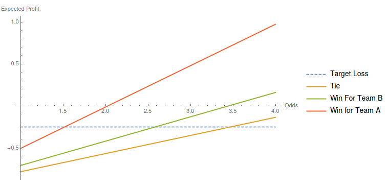
So far we haven’t talked about the betting odds. What we need is a positive expected profit for the betting company or negative for the client for every possible action of the client. If the client predicts that team $A$ will win, their expected winnings (per currency unit) will be:

$$\mathbb E[predict_A]= (w_A-1) \mathbb P[Goal_A>Goal_B] - (1-\mathbb P[Goal_A>Goal_B])$$ or simplified: $\mathbb E[predict_A]= w_A \mathbb P[Goal_A>Goal_B] - 1$

If the client predicts a draw their expected profit will be:

$$ \mathbb E[predict _{draw}]= (t-1) \mathbb P[Goal _A=Goal _B] - (1-\mathbb P[Goal _A=Goal _B])$$

or simplified: $\mathbb E[predict_{draw}]= t \mathbb P[Goal_A=Goal_B] - 1$

similarly: $\mathbb E[predict_B]= w_B \mathbb P[Goal_A<Goal_B] - 1$

Given that, the Betting company would have to set those odds so that the expected values will be negative but in a reasonable range. Additionally setting all the expected profits equal will make, in principle, every option equally enticing preventing imbalance in the number of bets in each option.

Example

I implement the analysis in Mathematica where we can skip the direct implementation of some parts since the language does that for you. The following function in Mathematica will compute the probability of team A winning, a tie, or team B winning.

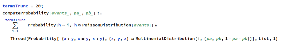
I truncate after 20 terms but this should depend on the mean number of events (or highlights). For example I get:

$$computeProbability[10, 0.2, 0.15]=\{0.492633, 0.215924, 0.289809\}$$

Changing $termsTrunc$ to $30$ results in very slightly modified probabilities, $\{0.493562, 0.216138, 0.290255\}$

Now If we decide to target a specific expected loss for the players, say $0.25$ currency units per 1 currency unit bet, we would choose roughly the following odds as seen in the plot: $1.5$ for win of team A, $2.6$ for win of team B, $3.5$ for a tie. How high or low this target loss is another topic that deserves a seperate study.

References & Links

1. Multinomial Distribution
2. Simulating the Poisson Process, PATRICK MCQUIGHAN
3. Quality of Experience